

Here is the basic process for Bayesian reasoning:
Start with a prior. A probability distribution over hypothesis space that represents your starting beliefs.
Make an observation $B$.
Scale the prior pointwise by each hypothesis' predicted probability of $B$.
Normalize the prior so it adds up to 100%. This is your new posterior.
Goto 2.
One of the problems you run into right away, when implementing this in a computer program, is "How do I pick the prior?". A good rule of thumb is to just assign each hypothesis equal likelihood, but this breaks down in cases where there are infinitely many possible hypotheses. The probabilities-must-add-up-to-100% requirement forces you to compute $\infty/\infty$, which is undefined, and all the math gears seize up.
There are many reasonable workarounds for this problem, but I want to discuss one that I came up with: just saying "screw normalization!". (Actually, as per usual, I quickly found out my idea was in no way original. Improper priors are a century-old tool that I should have known about before starting this post... but here we are regardless.)
Suppose, for the sake of argument, that we started the Bayesian inference process with a distribution that wasn't a probability distribution. What happens? Let's do an example to see.
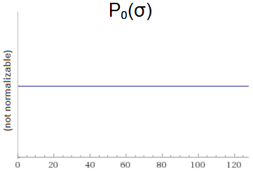
Suppose we are sampling from a normal distribution. We know that the mean of the distribution is $\mu=0$, but we don't know the standard deviation $\sigma$. We want to use Bayesian reasoning to infer $\sigma$, so we need a prior. We decide to use the improper uniform prior $P_0(\sigma) = 1$ for $\sigma \in (0, \infty)$:
Now we do an inference step. We sample $x_1$ from the distribution, and find that $x_1=6$.
Given a hypothesized $\sigma$, the probability of sampling $x_1=6$ is $\mathcal{N}_{0, \sigma}(6)$. That means our posterior is:
$$\begin{align} P_1(\sigma) &\propto P_0(\sigma) \cdot \mathcal{N}_{0, \sigma}(6) \\ &= 1 \cdot \frac{\exp\left( -6^2 / 2 \sigma^2 \right)}{\sigma \sqrt{\tau}} \\ &= \frac{\exp\left( -18 / \sigma^2 \right)}{\sigma \sqrt{\tau}} \end{align}$$
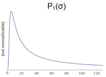
Note that we didn't normalize. That's because we can't. This is still a malformed distribution. The numerator of $P_1$ converges to 1, but the denominator makes the expression act like $1/\sigma$. So the overall the cumulative distribution will diverge like $\Theta(\lg \sigma)$.
Things are still broken after one observation, but they're not as broken. We used to be diverging linearly, but now we're only diverging logarithmically. Maybe another sample will do the trick?
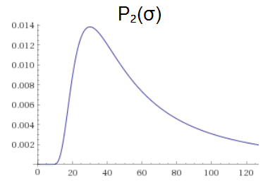
We sample again, find that $x_2=42$, and compute the posterior:
$$\begin{align} P_2(\sigma) &\propto P_1(\sigma) \cdot \mathcal{N}_{0, \sigma}(42) \\ &= \frac{\exp\left( -18 / \sigma^2 \right)}{\sigma \sqrt{\tau}} \cdot \frac{\exp\left( -42^2 / 2 \sigma^2 \right)}{\sigma \sqrt{\tau}} \\ &= \frac{\exp\left( -18 / \sigma^2 \right)}{\sigma \sqrt{\tau}} \cdot \frac{\exp\left( -882/ \sigma^2 \right)}{\sigma \sqrt{\tau}} \\ &= \frac{\exp\left( -30^2/ \sigma^2 \right)}{\sigma^2 \tau} \end{align}$$
Now that the denominator is squared, the cumulative distribution converges to a finite number:
$$\int_0^\infty \frac{\exp\left(-30^2/ \sigma^2 \right)}{\sigma^2 \tau} d\sigma = \frac{1}{120 \sqrt{\pi}} \approx 0.0047$$
And we can get a proper posterior probability distribution by using this cumulative total to renormalize:
$$ P_2(\sigma) =\frac{60 \exp\left(-30^2/ \sigma^2 \right)}{\sigma^2 \sqrt{\pi}} $$
Although we started with a meaningless prior, the updating process eventually brought us back into the space of well-formed probability distributions. This is kind of nice, because $P(x) = 1$ is a very simple prior. It doesn't even take any parameters! Sure it forces some minimum number of observations before you're able to get a meaningful prediction, but it's not like other uninformed priors were going to score well on metrics before being updated by observations.
In fact, I think this concept of improper prior justifies a lot of frequentist statistics. A good example is what happens when you estimate the true mean of a population by sampling. A frequentist calculation creates a distribution of possible means exactly centered on the sampled mean. But a hard-core literal Bayesian would start with a prior, and that prior would bias the posterior away from being centered exactly on the sampled mean... unless you started with the improper prior $\forall \mu, P(\mu) = 1$.
Do be careful, though. You can create some pretty crazy improper priors. For example, consider $P(x) = e^{x^2}$ for $x \in (-\infty, +\infty)$. A Bayesian computer program initialized with such a prior would have what I can only describe as an unbreakable faith in the infinite. No matter how many normally-distributed observations you fed in, you'd never get a proper probability distribution out.
In addition to the prior being too wild, the updating process may be too weak or the hypothesis space may be too complicated. For example, even a nearly-converging prior like $P(x) = 1/x$ will cause serious problems for Solomonoff induction.
Summary
By definition, Bayesian priors are probability distributions. But violating that definition leads to interesting and useful behaviors.
